
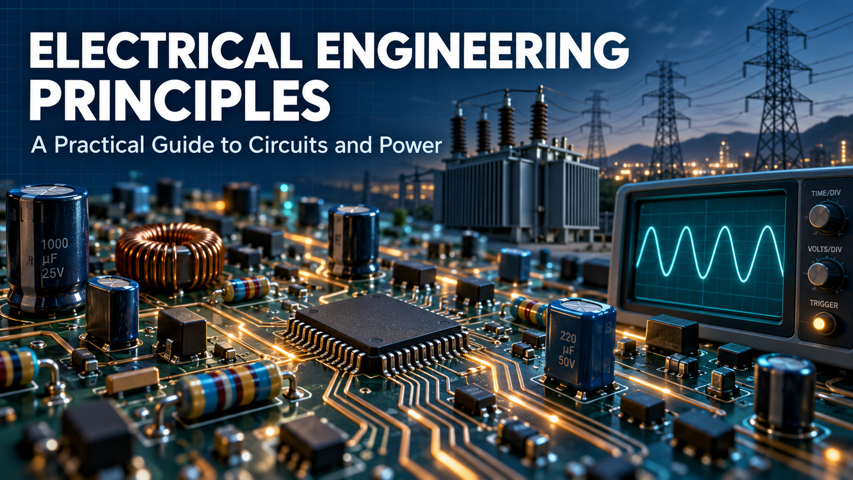
Electrical engineering principles explain how charge, current, energy, and electromagnetic fields behave. Engineers use them to analyze circuits, select components, understand machines, and check whether a design can perform reliably under its intended conditions.
Why does a motor draw more current during startup? Why can a circuit pass a continuity check and still fail under load? What does power factor tell you that a watt rating does not?
You can answer these questions by connecting a few fundamental relationships to the actual equipment. Start with the source, follow the current path, identify where energy goes, and check the assumptions behind each calculation.
Consider a control device that operates correctly on a workbench but resets after installation. The device itself may work as intended. Resistance in a longer cable or a brief dip in the supply during startup could explain the behavior. Applying Engineering Principles helps you weigh safety, reliability, cost, and performance throughout the electrical design process.
Good analysis examines the complete circuit, including conditions that a nominal rating does not describe.
Electrical Fundamentals: Charge, Current, and Circuit Laws
Start with the quantities that describe a circuit. Current measures the rate at which charge passes a point. Voltage describes the electric potential difference between two points. Resistance describes opposition to current in a resistive element.
The distinction between a point and a pair of points matters. A statement such as “this terminal is at 24 volts” assumes a reference. Without that reference, the statement is incomplete.
| Quantity | Symbol | Common unit | What it describes |
| Charge | q | Coulomb, C | Quantity of electric charge |
| Current | I | Ampere, A | Rate of charge flow |
| Potential difference | V | Volt, V | Energy difference per unit charge |
| Resistance | R | Ohm, Ω | Opposition to current in a resistive element |
| Power | P | Watt, W | Rate of energy transfer |
| Energy | E | Joule, J, or kilowatt-hour, kWh | Accumulated energy transferred or used |
For an ideal resistor, Ohm’s law relates the applied potential difference, current, and resistance:
V=IRV = IR
Here, V describes the difference across the resistor, and I describes the current through it. The relationship assumes an appropriate resistive model. Diodes and many other devices do not behave like constant resistances over their operating range. OpenStax explains this distinction in its discussion of Ohm’s law.
Worked example: An ideal 12-volt DC source supplies a 6-ohm resistor. The current equals 12 divided by 6, or 2 amperes. The resistor dissipates 24 watts because P = VI.
For the same resistor, P = I²R and P = V²/R give the same answer. These alternative forms are useful only when the quantities refer to the same element and the resistive assumptions apply.
Kirchhoff’s current law balances current at a node. In the usual circuit model, the total entering equals the total leaving. If 5 amperes enters a junction and one branch carries 2 amperes away, the remaining branches must carry a combined 3 amperes away.
Kirchhoff’s voltage law balances the algebraic sum of potential changes around a closed loop. Use a consistent direction and sign convention. In circuits involving changing magnetic flux, represent the induced electromotive force appropriately rather than ignoring it.
Series components carry the same current. Parallel branches connect across the same two nodes and share the same potential difference. That topology determines which relationships you can use.
Two 10-ohm resistors in series produce 20 ohms. The same resistors in parallel produce 5 ohms. With a fixed ideal source, the arrangements draw different currents and dissipate different total power.
An open circuit interrupts the conducting path. A short circuit creates an unintended low-impedance path that can produce a large fault current. The available current depends on the source and the complete path, not simply on a component’s normal operating rating.
These principles of electricity provide a starting point. Real conductors, connections, and power supplies add resistance, limits, and temperature effects that the simplest model leaves out.
Data Engineering Principles help you organize and validate sensor readings, power measurements, and equipment records so you can trust the data behind your electrical design decisions.
Understanding AC Power, Energy Storage, and Electromagnetism
Direct current maintains one direction, although its magnitude can vary. Alternating current reverses direction periodically. Many introductory calculations assume sinusoidal waveforms because they make frequency and phase relationships easier to describe.
Frequency measures cycles per second in hertz. Phase describes the relative timing of waveforms. Two quantities can share the same frequency while reaching their peaks at different times.
For a sine wave, the root-mean-square value equals the peak divided by the square root of two. RMS provides a useful comparison of heating in a resistor. A 120-volt RMS sine wave has a peak of approximately 170 volts.
Capacitors and inductors introduce energy storage. A capacitor stores energy in an electric field; an inductor stores energy in a magnetic field. Their behavior depends on time and frequency, so constant resistance alone cannot describe them.
For ideal components in sinusoidal steady state, capacitive reactance has magnitude 1/(2πfC), while inductive reactance equals 2πfL. Increasing frequency reduces the former and increases the latter. These relationships help explain filters, startup behavior, and frequency-dependent responses.
Impedance combines resistance with reactance. It describes both magnitude and phase relationships in an AC circuit. Phasor methods make these calculations manageable when the circuit and operating assumptions support them.
Power versus energy: Power describes a rate. Energy accumulates over time. A constant 2-kilowatt load operating for three hours uses 6 kilowatt-hours. A kilowatt-hour is a unit of energy, despite having “watt” in its name.
For single-phase AC, real power equals RMS potential difference multiplied by RMS current and power factor. Apparent power is the product of the two RMS magnitudes, expressed in volt-amperes. For sinusoidal waveforms, power factor equals the cosine of the phase angle between them. See OpenStax’s explanation of AC power.
Suppose a load draws 10 amperes from a 120-volt RMS source at a power factor of 0.80. Apparent power is 1,200 volt-amperes, while real power is 960 watts.
Do not confuse power factor with efficiency. Efficiency compares useful output with input power. Power factor compares real power with apparent power. A motor can have different values for each.
Electromagnetism connects circuit behavior with transformers and machines. Changing magnetic flux induces an electromotive force. In a conventional transformer, this interaction transfers energy between windings; applying steady DC does not produce normal continuous transformer operation.
Motors convert supplied energy into mechanical work while losses produce heat. Startup current can differ substantially from running current because the machine has not yet reached its normal operating state. The details depend on the motor and starting method.
A transient describes behavior during a transition. In an ideal resistor-capacitor charging circuit, the time constant equals resistance multiplied by capacitance. After one time constant, a capacitor initially at zero reaches about 63 percent of its final potential under a step input.
For a 10,000-ohm resistor and a 100-microfarad capacitor, the time constant is one second. Reaching the final value takes more than one time constant; after five, the ideal response reaches about 99.3 percent.
This example explains why a circuit can behave differently immediately after switching and several seconds later. It also shows why stored energy matters: disconnecting a source does not necessarily remove the energy already held in a capacitor.
Electrical engineering therefore examines steady operation, transitions, and faults. One nameplate number cannot describe all three. Geotechnical Engineering Principles matter when substations and transmission structures need foundations that can handle equipment loads and local soil conditions.
From Circuit Board to Motor: Applying the Fundamentals
A useful calculation answers a specific question. Before choosing an equation, identify the operating condition and the behavior you need to establish.
For a control circuit, the question might be whether the device receives enough supply potential during its highest demand. For a motor, it might concern starting behavior, thermal loading, or the effect of a changing mechanical load.
Use a repeatable approach:
- Define the required behavior and operating range.
- Draw the complete path, including the return connection and source limits.
- Select a model that represents the important effects.
- Calculate the expected result and check units and magnitude.
- Compare the prediction with suitable specifications or verified measurements.
Return to the control device that resets after installation. For an illustrative steady-state calculation, suppose a nominal 24-volt DC source feeds a 2-ampere load through conductors with a combined outgoing-and-return resistance of 0.8 ohm.
The conductors drop 1.6 volts, leaving approximately 22.4 volts at the load. They dissipate 3.2 watts. That result assumes the source holds 24 volts and the load draws a constant 2 amperes.
If startup demand rises, the drop may increase. Some regulated loads respond differently as their input falls, so the constant-current assumption may no longer represent the equipment. Check the actual device characteristics before extending the example.
Thermal limits require similar care. In the earlier resistor example, 24 watts of dissipation does not mean that any resistor labeled 24 watts will suit the installation. Ambient temperature, mounting, airflow, and the manufacturer’s derating requirements influence allowable operation.
On a circuit board, conductor geometry and return paths can affect heating, noise, and signal behavior. At higher frequencies or with fast switching edges, interconnection details may become important enough that an ideal lumped model no longer captures the behavior adequately.
Component tolerance also matters. A nominal resistance, capacitance, or threshold represents a value with specified variation. Examine combinations that could affect performance instead of assuming every component sits exactly at its nominal value.
A sensitivity check helps identify the assumptions worth confirming first. If a small increase in conductor resistance puts the load below its permitted input range, temperature and connection condition deserve closer attention. If the result remains comfortably within limits across credible variations, another issue may deserve priority.
Document the range you examined. A calculation based on nominal conditions alone answers a narrower question than an evaluation covering expected operating extremes. Neither should imply that you investigated conditions you did not actually consider.
Measurement adds its own limitations. A meter’s input impedance can affect the circuit it observes. Instrument range, bandwidth, and accuracy must suit the signal and the intended conclusion. A stable display does not guarantee an accurate interpretation.
Protection needs an understanding of both normal operation and available fault energy. Grounding and bonding have distinct purposes, and a protective device must suit the installation and the faults it needs to interrupt. A basic load calculation alone does not establish a compliant installation.
For learning, use simulation and appropriately supervised, current-limited training equipment. Work on hazardous-energy equipment requires qualified personnel and procedures appropriate to the task. The calculations here explain behavior; they do not provide an energized-work procedure.
The best electrical engineering analysis ends with a clear statement: what the model predicts, which assumptions support it, and what additional evidence the decision requires.
Frequently Asked Questions
What should beginners learn first?
Start with charge, current, potential difference, resistance, power, and energy. Then practice series and parallel circuits, node and loop equations, and basic capacitor and inductor behavior.
Draw each circuit before calculating. Mark reference directions, write units through intermediate steps, and check whether the result makes physical sense. A negative current may simply mean the actual direction opposes your chosen reference.
A reliable electrical engineering reference should explain assumptions alongside equations. When using textbook pages or a PDF, work through examples independently rather than relying only on final answers.
Is EE the hardest degree, and what makes it difficult?
There is no objective ranking that makes electrical engineering the hardest degree for everyone. Its difficulty often comes from combining abstract models, mathematics, and physical behavior that you cannot directly observe.
Calculus, differential equations, complex numbers, and probability appear in different subjects. The challenge becomes more manageable when you connect each mathematical tool to a specific question, such as predicting a transient response or interpreting a signal.
What are the eight main types of electrical engineering?
There is no single official eight-part classification. A useful overview includes power and energy, electronics, control, communications, signal processing, electromagnetics, microelectronics, and computer hardware.
The boundaries overlap. A motor drive combines power conversion, control, sensing, and embedded computing. Universities and employers group these specialties differently, so examine the actual coursework or responsibilities behind a title.
Can you make $500,000 as an electrical engineer?
That level of annual compensation is possible in exceptional circumstances, such as senior leadership, highly compensated specialist roles with substantial equity, or successful business ownership. It is not a typical salary expectation for the occupation.
Distinguish base salary from bonuses, stock compensation, and business income. The Bureau of Labor Statistics occupational profile provides a more useful starting point for understanding typical pay than unusually high individual compensation reports.
How can you turn theory into practical skill?
Choose a small circuit and predict its behavior before simulating or testing it. Compare the result with your prediction, then vary one input or component value and explain the difference.
That cycle builds judgment. You learn which assumptions matter, where an ideal model works, and when the actual equipment requires a more detailed explanation.